Maximum Likelihood Estimation of Weibull reliability with DiffSharp

28 Aug 2022

This post is a continuation of my exploration of DiffSharp, an F# Automatic Differentiation library. In the previous post, I covered some introductory elements of Maximum Likelihood Estimation, through a toy problem, estimating the likelihood that a sequence of heads and tails had been generated by a fair coin.

In this post, I will begin diving into the real-world problem that motivated my interest.

The general question I am interested in is about reliability. Imagine that you have a piece of equipment, and that from time to time, a component of that piece of equipment experiences failures. When that happens, you replace the defective component with a new one, restart the equipment, and proceed until the next failure.

The log for such a process would then look something like this:

Jan 07, 2020, 08:37  Component failure
Jan 17, 2020, 13:42  Component failure
Feb 02, 2020, 06:05  Component failure
Feb 06, 2020, 11:17  Component failure

If you wanted to make improvements to the operations of your equipment, one useful technique would be to simulate that equipment and its failures. For instance, you could evaluate a policy such as “we will pre-emptively replace the Component every week, before it fails”. By simulating random possible sequences of failures, you could then evaluate how effective that policy is, compared to, for instance, waiting for the failures to occur naturally.

However, in order to run such a simulation, you would need to have a model for the distributions of these failures.

The log above contains the history of past failures, so, assuming nothing changed in the way the equipment is operated, it is a sample of the failure distribution we are interested in. We should be able to use it, to estimate what parameters are the most likely to have generated that log. Let’s get to it!

Environment: dotnet 6.0.302 / Windows 10, DiffSharp 1.0.7

Full code on GitHub

Weibull time to failure

What we are interested in here is the time to failure, the time our equipment runs from the previous component replacement to its next failure. A classic distribution used to model time to failure is the Weibull distribution.

The Weibull distribution is not the only option available, but it has interesting properties. It is a continuous probability distribution, over positive numbers, and is defined by 2 parameters, one describing its shape, k, the other its scale, lambda. Let’s examine these properties, through an F# code implementation:

type Weibull = {
    Lambda: float
    K: float
    }
    with
    member this.Density (x: float) =
        if x <= 0.0
        then 0.0
        else
            (this.K / this.Lambda)
            *
            (x / this.Lambda) ** (this.K - 1.0)
            *
            exp ( - ((x / this.Lambda) ** this.K))
    member this.Cumulative (x: float) =
        if x <= 0.0
        then 0.0
        else
            1.0
            -
            exp ( - ((x / this.Lambda) ** this.K))
    member this.InverseCumulative (p: float) =
        this.Lambda 
        *
        ( - (log (1.0 - p))) ** (1.0 / this.K)

Let’s examine the impact of the two parameters lambda and k graphically, using Plotly.NET:

#r "nuget: Plotly.NET.Interactive, 3.0.0"
open Plotly.NET

First, let’s plot the cumulative distribution for 3 values of lambda, 0.5, 1.0 and 2.0:

[ 0.5; 1.0; 2.0 ]
|> List.map (fun shape -> 
    let weibull = { Lambda = shape; K = 1.0 }
    [ 0.0 .. 0.1 .. 5.0 ]
    |> List.map (fun t -> t, weibull.Cumulative t)
    |> fun data -> Chart.Line(data, Name = $"Lambda = {shape}")
    )
|> Chart.combine
|> Chart.withXAxisStyle "Time to failure"
|> Chart.withYAxisStyle "Cumulative probability"
|> Chart.withTitle "Weibull: impact of scale parameter Lambda"

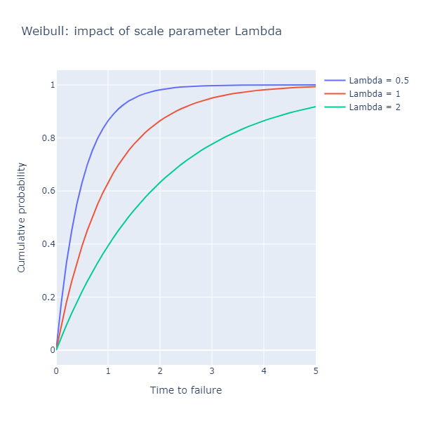
Weibull cumulative for different values of lambda

What the chart shows is the probability that after a certain amount of time has elapsed, the component has failed already. The scale parameter lambda stretches the curve: for lambda = 0.5, it will take half the time it takes a process with lambda = 1.0 to reach the same probability of having failed already. In other words, a lower value of lambda describes a process that fails faster.

How about the shape parameter k? Let compare 3 values, 0.5, 1.0 and 2.0:

[ 0.5; 1.0; 2.0 ]
|> List.map (fun k -> 
    let weibull = { Lambda = 1.0; K = k }
    [ 0.0 .. 0.1 .. 5.0 ]
    |> List.map (fun t -> t, weibull.Cumulative t)
    |> fun data -> Chart.Line(data, Name = $"K = {k}")
    )
|> Chart.combine
|> Chart.withXAxisStyle "Time to failure"
|> Chart.withYAxisStyle "Cumulative probability"
|> Chart.withTitle "Weibull: impact of shape parameter K"

Weibull cumulative for different values of k

The parameter k describes the overall shape of the distribution, and has important implications:

k = 1.0: the failure rate is constant over time (Weibull reduces to an Exponential distribution)
k < 1.0: the failure rate decreases over time, or, equivalently, we have a high rate of early failures (“infant mortality”),
k > 1.0: the failure rate increases over time, for instance for equipment that degrades with age.

As a result, the Weibull distribution is a good candidate to model failures, because it can represent a wide range of real-world behaviors, with just 2 parameters. The drawback, though, is that unlike the earlier example of the coin toss, there is no closed-form solution to estimate the parameters k and lambda given sample data.

Grid search estimation of Weibull failure parameters

Before bringing in the heavy machinery with DiffSharp, let’s get warmed up with solving the problem using grid search.

What we are trying to do here is to find the parameters k and lambda of a Weibull distribution that are the most likely to have generated a log of failures. In other words, we take as given that the underlying process is a Weibull distribution, and want to find the parameters that would fit the data best.

First, we need to transform the log a little. The original log example showed failures and their timestamp. What we are interested in is not timestamps, but time between failures. Let’s assume that we have done that transformation, which leaves us with a “tape” of time spans between consecutive failures.

In order to validate that our approach works, we need some benchmark. Again, we will use simulation: we will take a Weibull distribution, with set parameters, and use it to simulate a sequence of failures. As a result, we will be able to check how far off our estimates are from the true values of the parameters that actually generated that sample.

First, let’s simulate a tape:

let simulate (rng: System.Random, n: int) (weibull: Weibull) =
    Array.init n (fun _ ->
        rng.NextDouble ()
        |> weibull.InverseCumulative
        )

let rng = System.Random(0)
let sample =
    { Lambda = 0.8; K = 1.6 }
    |> simulate (rng, 100)

sample

For illustration, the first 5 results of that simulation look like this:

9405168968236842
1146238390817407
0139531031208946
7049619724501476
3198973954704749

What this tape represents is a first failure after 0.9405 units of time, followed by another after 1.1146 units of time, and so on and so forth.

We can now write a grid search over the combination of parameters k and lambda that maximizes the log-likelihood, like so:

[
    for lambda in 0.1 .. 0.1 .. 2.0 do
        for k in 0.1 .. 0.1 .. 2.0 do
            let w = { Lambda = lambda; K = k }
            (lambda, k),
            sample 
            |> Array.sumBy (fun t -> 
                log (w.Density(t))
                )
]
|> List.maxBy snd

We search for all combinations of k and lambda between 0.1 and 2.0, by increments of 0.1. For each combination, we create the corresponding Weibull, and compute the log likelihood that this particular distribution has generated the sample observations (the sum of the logarithms of the corresponding Weibull density), and return the combination that gives us the largest log likelihood.

In this example, we get lambda = 0.9, k = 1.6, which is decently close to the true parameters we used to generate the sample, lambda = 0.8, k = 1.6. In other words, the method seems to work.

Using DiffSharp to estimate the Weibull failure parameters

Grid seach has the benefit of simplicity, but has also drawbacks. First, as mentioned in the previous post, the space of combinations we need to explore grows fast with the number of parameters. In this case, we are exploring 20 values per parameter, or 20 x 20 = 400 combinations for 2 parameters. If we were interested in n parameters, we would have to generate 20 ^ n combinations, which is not ideal. Furthermore, we capped the search at a maximum value of 2.0 - but in general, k or lambda could take any positive value, and if these happened to be higher than 2.0, we would miss them.

Let’s use automatic differentiation with DiffSharp instead! We will follow more or less the same path as in the previous post, creating the log-likelihood function in F#, and using gradient ascent to find its maximum value by changing the 2 parameters k and lambda.

Rather than reiterating the whole process, I will just highlight the differences here. The only meaningful change is in the probability model itself:

let probabilityModel () =

    // We start with an initial guess for our Weibull,
    // with lambda = 1.0, k = 1.0.
    let lambda =
        1.0
        |> dsharp.scalar
        |> Parameter
    let k =
        1.0
        |> dsharp.scalar
        |> Parameter

    let parameters =
        [| lambda; k |]

    // We create the Probability Density function,
    // specifying that we want to differentiate it
    // with respect to the Lambda and K parameters.
    differentiable
        parameters
        (fun (time: float) ->
            if time <= 0.0
            then dsharp.scalar 0.0
            else
                (k.value / lambda.value)
                *
                ((time / lambda.value) ** (k.value - 1.0))
                *
                (exp ( - ((time / lambda.value) ** k.value)))
            )

We initialize the algorithm with a starting guess for a Weibull distribution with parameters lambda = 1.0, k = 1.0, and rewrite the Weibull density function we had earlier, as a function of these two parameters, so we can compute its partial derivative with respect to these 2 parameters.

And… that’s pretty much it. We can leave the maximizeLikelihood function we wrote last time unchanged, plug in our simulated sample, and wait for the magic to happen:

let config = {
    LearningRate = 0.001
    MaximumIterations = 100
    Tolerance = 0.001
    }

let rng = Random 0

let sample =
    { Lambda = 1.5; K = 0.8 }
    |> simulate (rng, 100)

probabilityModel ()
|> maximizeLikelihood config sample

… which produces the following estimates:

lambda = 1.8769636154174805, k = 0.8026720285415649

For completeness, we can write a small harness, generating multiple samples for different Weibull distributions, to evaluate how good or bad the estimates are:

let evaluation (rng: Random) (weibull: Weibull) =
    let sample =
       weibull
        |> simulate (rng, 100)
    let estimate =
        probabilityModel ()
        |> maximizeLikelihood config sample
    estimate

Array.init 10 (fun _ ->
    let lambda = 0.5 + 2.0 * rng.NextDouble()
    let k = 0.5 + rng.NextDouble()
    let weibull = { Lambda = lambda; K = k }
    weibull, evaluation rng weibull
    )

In general, the estimates do not exactly match the true values, which is expected. However, they fall fairly close. The one thing I noticed (and this might be a fluke, given the relatively small sample size) is that the estimates for lambda, the scale parameter, appeared to be less reliable for larger values of lambda.

Conclusion and Parting Notes

Enough for today! If you are interested in looking at the full code, here is a link to the .NET interactive notebook on GitHub.

Not many comments or thoughts this time. Going from the toy problem of the coin to a more complex one was actually very straightforward. The only work required was to express the Weibull density function as a DiffSharp function, which was not difficult at all. For that matter, it seems that it should be possible to make the code more easily re-usable. All we need for Maximum Likelihood Estimation is a density function, which can be applied to the sample observations, so if we had a sample like seq<'Obs>, the density should be constrained to be of the form Model<'Obs, float> (where the float is a probability).

Next time, we will keep exploring reliability problems, taking on a more complex situation: what if instead of a single source of failure, we had multiple competing ones?

Anyways, hope you found this post interesting! Ping me on Twitter if you have comments or questions, and… happy coding!

Do you have a comment or a question?
Ping me on Mastodon!