
Support Vector Machine: work in progress
25 Nov 2012Machine Learning in Action, in F#
Porting Machine Learning in Action from Python to F#
- KNN classification (1)
- KNN classification (2)
- Decision Tree classification
- Naive Bayes classification
- Logistic Regression classification
- SVM classification (1)
- SVM classification (2)
- AdaBoost classification
- K-Means clustering
- SVD
- Recommendation engine
- Code on GitHub
I am still working my way through “Machine Learning in Action”, converting the samples from Python to F#. I am currently in the middle of chapter 6, dedicated to Support Vector Machines, which has given me more trouble than the previous ones. This post will be sharing my current progress: the code I have so far is a working translation of the naïve SVM implementation, presented in the first half of the chapter. We’ll get to kernels, and the full Platt SMO algorithm in a later post - today will be solely discussing the simple, un-optimized version.
Two factors slowed me down with this chapter: the math, and Python.
The math behind the algorithm is significantly more involved than the other algorithms, and I won’t even try to go into why it works. I recommend reading An Idiot’s guide to SVMs, which I found a pretty complete and accessible explanation of the theory behind SVMs. I will focus instead on the implementation, which was in itself a bit challenging.
First, the Python code uses algebra quite a bit, and I found that deciphering what was going on required a bit of patience. Take a line like the following:
fXi = (float)(multiply(alphas, labelMat).T*(dataMatrix*dataMatrix[i,:].T))+b
I am reasonably well versed in linear algebra, but figuring out what this is saying takes some attention. Granted, I have no experience with Python and NumPy, so my whining is probably a bit unfair. Still, I thought the code was not very readable, and it motivated me to see if that could be improved, and as a result I ended up moving away from heavy algebra notation.
Then, the algorithm is implemented as a Deep Arrow. A main loop performs computations and evaluates conditions at multiple points, using continue to exit / short-circuit the evaluation. The code I ended up with doesn’t use mutation, but is still heavily indented, which I am not happy about - I’ll work on that later.
Simplified algorithm implementation
Note: as the title of the post indicates, this is work in progress. The current implementation works, but has some obvious flaws (see last paragraph), which I intend to fix in upcoming posts. My intent is to share my progression through the problem - please don’t take this as a good reference SVM implementation. Hopefully we’ll get there soon, but this is not it, not yet.
You can find the code discussed below on GitHub.
Enough said - let’s go into the algorithm. We are trying to solve essentially the same problem we described with Logistic Regression: we have a set of observations, where each observation belongs to one of two groups, and data consists of numeric measurements on multiple dimensions. We want to use them to train a classifier, to predict what group new observations belong to.
For the time being, we’ll assume that the dataset is linearly separable - that is, there is a plane (or, in 2 dimensions, a line) such that all observations of one group are on one side, and of the other group on the other. Unlike for Logistic Regression, the groups are denoted by 1 and - 1; as a result, we want a classifier that returns a number: close to 0 is uncertain, large distances from 0 indicate “confident” classification, and the predicted group is identified by the sign of the number.
In a nutshell, here is what the algorithm does: it searches for observations from our dataset that are closest to the decision boundary (the plane), the support vectors, and assigns positive weights alpha to each support vector. The alphas and labels are used as weights to create a linear combination of the support vectors (itself a vector), which, together with a constant term b, defines the separating plane. The algorithm attempts to optimize b and the alpha coefficients so that the decision boundary has the largest possible margin from the support vectors (the next section of this post contains a few charts showing results of the algorithm in action, which may help visualize). Let’s go through the key elements of the current implementation, which you will find in the SupportVectorMachine module. I took a bit of a departure from the Python code; instead of using matrices and vectors, I created a simple SupportVector type:
type SupportVector = { Data: float list; Label: float; Alpha: float }
Data is the vector corresponding to an observation, which we model as a simple list of floats. The core of the simplified algorithm looks like this:
let simpleSvm dataset labels parameters =

    let size = dataset |> List.length
    let b = 0.0

    let rows =
        List.zip dataset labels
        |> List.map (fun (d, l) -> { Data = d; Label = l; Alpha = 0.0 })

    let rng = new Random()
    let next i = nextAround size i

    let rec search current noChange i =
        if noChange < parameters.Depth
        then
            let j = pickAnother rng i size
            let updated = pivot (fst current) (snd current) parameters i j
            match updated with
            | Failure -> search current (noChange + 1) (next i)
            | Success(result) -> search result 0 (next i)
        else
            current

    search (rows, b) 0 0
It has the following signature:
val simpleSvm : float list list -> float list -> Parameters -> SupportVector list * float
In plain English, what it says is that it expects a list of list of floats (the observations), a list of floats (the labels for each observation), and Parameters - and produces a list of SupportVector, and a float (the constant b).
The body of the algorithm is relatively straightforward: we initialize b to 0, and create a support vector for each observation of the dataset, initializing alphas to 0. We then declare a recursive function search, which perpetually cycles over the rows (using the next function), selects a random second row (using the selectAnother function), and attempts to “pivot” the 2 rows together. If the pivot succeeds, the 2 corresponding alphas get updated and we keep going, otherwise we increase the count of successive failed updates - and we stop when the count of successive failed updates reaches a user-defined number (parameters.Depth).
The ugly part of the algorithm is not-so-well hidden in the pivot function. Given 2 support vectors, and the current set of support vectors, pivot attempts to improve the alphas for the 2 support vectors and b, performing a few checks along the way, which may invalidate the pivot attempt. This is the deeply nested function I was mentioning earlier - it works, but it is ugly as hell, and its steps are a bit involved. I will invoke my right to hand-wave and won’t even attempt an explanation here, we’ll revisit it in a later post.

Instead, let’s go to the end of the algorithm, which produces the classifier:
let weights rows =
    rows
    |> Seq.filter (fun r -> r.Alpha > 0.0)
    |> Seq.map (fun r ->
        let mult = r.Alpha * r.Label
        r.Data |> List.map (fun e -> mult * e))
    |> Seq.reduce (fun acc row ->
        List.map2 (fun a r -> a + r) acc row )

let classifier (data: float list list) (labels: float list) parameters =
    let estimator = simpleSvm data labels parameters
    let w = weights (fst estimator)
    let b = snd estimator
    fun obs -> b + dot w obs
The classifier function expects the same arguments as the simpleSvm function: it reduces the support vectors retrieved from simpleSvm into a single vector w, the weighted sum of the support vectors (computed in a rather heavy-handed fashion in the weights function), and returns a function, with signature float list - > float. That function is the equation of the separating hyperplane: it will return 0 for observations lying on the plane, and respectively positive or negative values for observations belonging to group 1 or -1.
The algorithm in action
Let’s try the algorithm in a script, which you will find in the Chapter6.fsx file on GitHub. We’ll use FSharp.Chart to visualize what is happening in 2-dimensions problems.
Note: there are lots of ways the script could be improved. Frankly, my goal was to quickly validate whether the SVM code was working or not - so I went for quick rather than beautiful. shamelessly copy-pasting some of my older charting code.
Let’s create 2 datasets of random points, with X and Y coordinates between 0 and 100:
// tight dataset: there is no margin between 2 groups
let tightData =
    [ for i in 1 .. 500 -> [ rng.NextDouble() * 100.0; rng.NextDouble() * 100.0 ] ]
let tightLabels =
    tightData |> List.map (fun el ->
        if (el |> List.sum >= 100.0) then 1.0 else -1.0)

// loose dataset: there is empty "gap" between 2 groups
let looseData =
    tightData
    |> List.filter (fun e ->
        let tot = List.sum e
        tot > 110.0 || tot < 90.0)
let looseLabels =
    looseData |> List.map (fun el ->
        if (el |> List.sum >= 100.0) then 1.0 else -1.0)
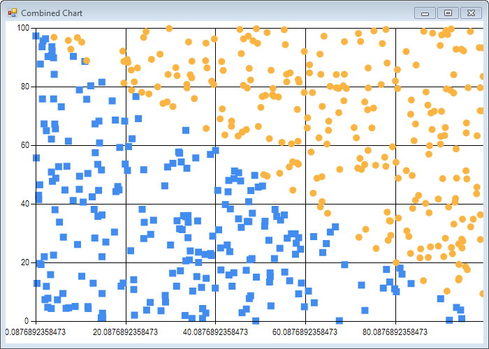
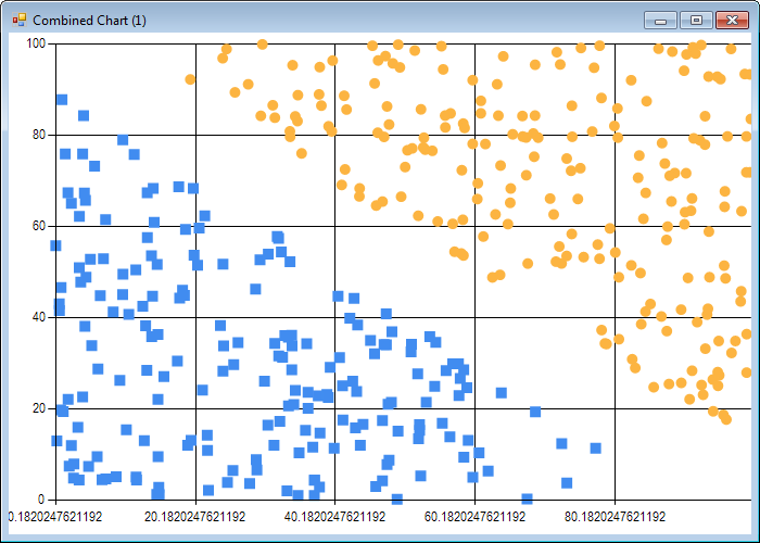
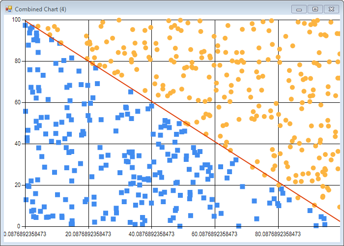
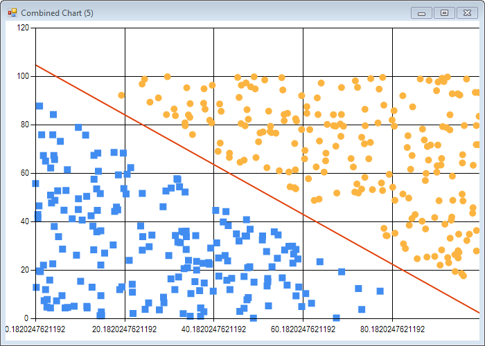
The first dataset is divided along the northwest - southeast diagonal: points such that X + Y > 100 are classified as 1, otherwise -1. By construction, our dataset is linearly separable. The second dataset is “loose”: we take the first dataset, and simply filter out points such that 90 < X + Y < 110, that is, observations that are close to the boundary.
Let’s visualize the two datasets:
// create an X,Y scatterplot, with different formatting for each label
let scatterplot (dataSet: (float * float) seq) (labels: 'a seq) =
    let byLabel = Seq.zip labels dataSet |> Seq.toArray
    let uniqueLabels = Seq.distinct labels
    FSharpChart.Combine
        [ // separate points by class and scatterplot them
          for label in uniqueLabels ->
               let data =
                    Array.filter (fun e -> label = fst e) byLabel
                    |> Array.map snd
               FSharpChart.Point(data) :> ChartTypes.GenericChart
               |> FSharpChart.WithSeries.Marker(Size=10)
        ]
    |> FSharpChart.Create

// plot raw datasets
scatterplot (tightData |> List.map (fun e -> e.[0], e.[1])) tightLabels
scatterplot (looseData |> List.map (fun e -> e.[0], e.[1])) looseLabels
Note that due to the algorithm inherent randomness, results will be slightly different each time you run the code.
Now let’s run the simpleSvm function, and visualize the support vectors identified by the algorithm:
let plot (data: float list list) (labels: float list) parameters =
    let estimator = simpleSvm data labels parameters
    let labels =
        estimator
        |> (fst)
        |> Seq.map (fun row ->
            if row.Alpha > 0.0 then 0
            elif row.Label < 0.0 then 1
            else 2)
    let data =
        estimator
        |> (fst)
        |> Seq.map (fun row -> (row.Data.[0], row.Data.[1]))
    scatterplot data labels

let parameters = { C = 0.6; Tolerance = 0.001; Depth = 500 }

plot tightData tightLabels parameters
plot looseData looseLabels parameters
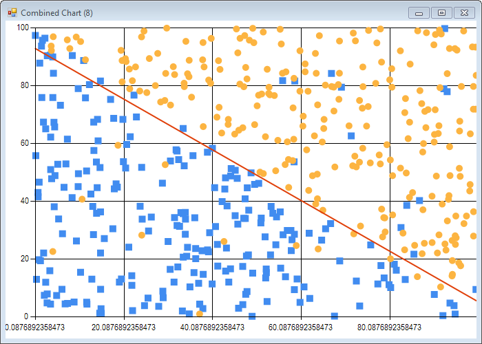
We run the simpleSvm function, and map the support vectors to 3 groups: 0 if alpha is greater than 0 (the observation has been selected as a support vector), and for the rest, 1 or 2 depending on the observation label:
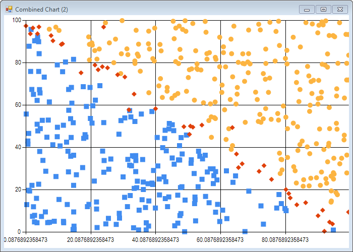
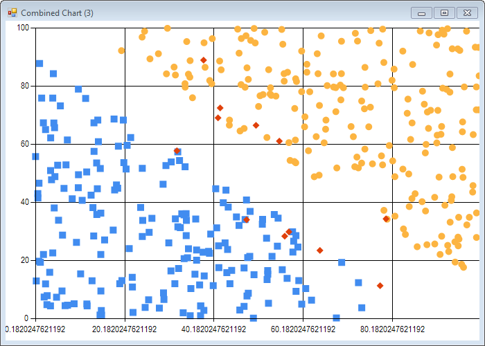
Obviously, the algorithm is doing something right - we see in both cases 2 big blocks of observations on the sides of the boundaries, and a smaller set of points bunched close to the boundary. It’s not perfect (some points are far off the boundary), but that’s expected from the algorithm, which is an approximation rather than a perfect solve.
Can we get a sense for the quality of the classifier? Sure we can:
let test (data: float list list) (labels: float list) parameters =
    let classify = classifier data labels parameters
    let performance =
        data
        |> List.map (fun row -> classify row)
        |> List.zip labels
        |> List.map (fun (a, b) -> if a * b > 0.0 then 1.0 else 0.0)
        |> List.average
    printfn "Proportion correctly classified: %f" performance

let parameters = { C = 0.6; Tolerance = 0.001; Depth = 500 }

test tightData tightLabels parameters
test looseData looseLabels parameters
We compute a classifier from the dataset, apply it to the observations, and count the proportion of proper classifications, that is, observations where the sign of the Label is the same as the sign of the Prediction. Here is my result:
Proportion correctly classified: 0.988000
Proportion correctly classified: 1.000000
Real: 00:00:00.906, CPU: 00:00:00.906, GC gen0: 10, gen1: 1, gen2: 0
Under 1 second, we get a near perfect classifier on a 500 observations dataset (note: yes, I should have trained the classifier on a subset of the data, and tested it on the rest).
Can we visualize the decision boundary? And why not:
// display dataset, and "separating line"
let separator (dataSet: (float * float) seq) (labels: 'a seq) (line: float -> float) =
    let byLabel = Seq.zip labels dataSet |> Seq.toArray
    let uniqueLabels = Seq.distinct labels
    FSharpChart.Combine
        [ // separate points by class and scatterplot them
          for label in uniqueLabels ->
               let data =
                    Array.filter (fun e -> label = fst e) byLabel
                    |> Array.map snd
               FSharpChart.Point(data) :> ChartTypes.GenericChart
               |> FSharpChart.WithSeries.Marker(Size=10)
          // plot line between left- and right-most points
          let x = Seq.map fst dataSet
          let xMin, xMax = Seq.min x, Seq.max x
          let lineData = [ (xMin, line xMin); (xMax, line xMax)]
          yield FSharpChart.Line (lineData)  :> ChartTypes.GenericChart
        ]
    |> FSharpChart.Create

let plotLine (data: float list list) (labels: float list) parameters =
    let estimator = simpleSvm data labels parameters
    let w = weights (fst estimator)
    let b = snd estimator
    let line x = - b / w.[1] - x * w.[0] / w.[1]
    separator (data |> Seq.map (fun e -> e.[0], e.[1])) labels line

plotLine tightData tightLabels parameters
plotLine looseData looseLabels parameters
This is essentially the same code as before - we just compute from the estimates the equation of the separating line, and add it to the chart:
I’ll leave it at that for this post; if you check the script Chapter6.fsx, there is a bit more material, like a noisy dataset, where some observations are misclassified. Be careful with that one: for obvious reasons, the algorithm runs much, much slower (a bit under 2 minutes on my PC), which is understandable, as the dataset is not linearly separable any more, which makes the job significantly harder.
Parting words
Again, this is work in progress - the algorithm in its current form, which you can find on GitHub, has a few obvious flaws:
The pivot function is really ugly. The attempt to produce an updated pair of Support Vectors can fail in four places which cause a premature exit, and still looks deeply indented, which is highly displeasing to the eye, and makes the code hard to follow. I am still not totally certain what the right approach is here, but suspect a Computation Expression is the way to go (probably along the lines of the Attempt Builder).
Given that the current implementation accesses Support Vectors by index, using a list is likely a bad idea, performance wise. I kept it that way for the moment because the full Platt SMO algorithm implementation is organized a bit differently. Rather than optimize for the naïve version, I prefer to wait until I understand better what the correct data structure is.
I think moving away from a pure matrix/vector representation, using a SupportVector record type instead, clarifies what is going on. On the other hand, the calculations and helper methods (notably what is taking place in the pivot function) are still fairly obscure, and feel like they are in an in-between state, half linear algebra and half operations on sets of SupportVectors. I got this nagging feeling that there is a better, simpler way to represent the whole algorithm and what it does - I just need to get past the original code, and hopefully at some point a simpler, more consistent design will emerge.
"The lurking suspicion that something could be simplified is the world’s richest source of rewarding challenges." -Dijkstra
— Scott Raymond (@sco) November 25, 2012
Somewhat relatedly, now that I am 5 chapters in the book, I can see some code duplication between my modules, the most obvious case being basic vector operations - I foresee some consolidation soon.
I am glad I wrote some unit tests - it helped me spot a minor typographical mistake (+ instead of - ), which was a major bug. The code is far from fully tested, though: most of it is perfectly testable, but some of the functions are nasty because they involve lots of conditions. I am hoping to see some simplification as the design matures.
That’s all I have for now - our next steps will be getting rid of the deep arrow, looking into Kernels, and implementing the full Platt SMO algorithm. Busy week-ends ahead!
As usual, I welcome comments, feedback and suggestions.
Additional resources
- Code in its current form on GitHub.
- An idiot’s guide to Support Vector Machines: very good and fairly accessible general exposition of SVMs.
- Support vector machines (SVMs) in F# using Microsoft Solver Foundation: excellent post, demonstrating how to explicitly solve the problem as a Quadratic Programming optimization problem, using F# and the Microsoft Solver Foundation.