
Logistic Regression
30 Sep 2012Machine Learning in Action, in F#
Porting Machine Learning in Action from Python to F#
- KNN classification (1)
- KNN classification (2)
- Decision Tree classification
- Naive Bayes classification
- Logistic Regression classification
- SVM classification (1)
- SVM classification (2)
- AdaBoost classification
- K-Means clustering
- SVD
- Recommendation engine
- Code on GitHub
After four weeks of vacations, I am back home, ready to continue my series of posts converting the samples from Machine Learning in Action from Python to F#.
Today’s post covers Chapter 5 of the book, dedicated to Logistic Regression. Logistic Regression is another classification method. It uses numeric data to determine how to separate observations into two classes, identified by 0 or 1.
The entire code presented in this post can be found on GitHub, commit 398677f
The idea behind the algorithm
The main idea behind the algorithm is to find a function which, using the numeric data that describe an individual observation as input, will return a number between 0 and 1. Ideally, that function will return a number close to respectively 0 or 1 for observations belonging to group 0 or 1.
To achieve that result, the algorithm relies on the Sigmoid function:
f(x) = 1 / (1 + exp(-x))
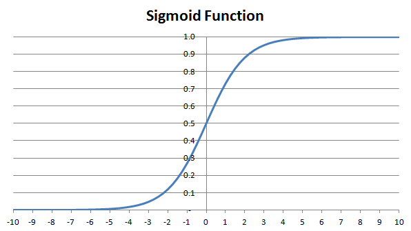
For any input value, the Sigmoid function returns a value in ] 0 ; 1 [. A positive value will return a value greater than 0.5, and the greater the input value, the closer to 1. One could think of the function as returning a probability: for very high or low values of x, there is a high certainty that it belongs to one of the two groups, and for values close to zero, the probability of each group is 50% / 50%.
The only thing needed then is a transformation taking the numeric values describing the observations from the dataset, and mapping them to a single value, such that applying the Sigmoid function to it produces results close to the group the observation belongs to. The most straightforward way to achieve this is to apply a linear combination: an observation with numeric values [ x1; x2; ... xk ] will be converted into w0 + w1 x x1 + w2 x x2 ... + wk x xk, by applying weights [ w0; w1; ... wk ] to each of the components of the observation.
Note how the weights have one extra element w0, which is used for a constant term.
If our observations had two components X and Y, each observation can be represented as a point (X, Y) in the plane, and what we are looking for is a straight line w0 + w1 x X + w2 x Y, such that every observation of group 0 is on one side of the line, and every observation of group 1 on the other side.
We now replaced one problem by another - how can we find a suitable set of weights W?
I won’t even attempt a full explanation of the approach, and will stick to fuzzy, high-level intuition. Basically, the algorithm starts with an arbitrary set of weights, and iteratively adjusts the weights, by comparing the results of the function and what it should be (the actual group), and adjusting them to reduce error.
Note: I’ll skip the Gradient Ascent method, and go straight to the second part of Chapter 5, which covers Stochastic Gradient Ascent, because the code is both easier to understand and more suitable to large datasets. On the other hand, the deterministic gradient ascent approach is probably clearer for the math inclined. If that’s your situation, you might be interested in this MSDN Magazine article, which presents a C# implementation of the Logistic Regression.
Let’s illustrate the update procedure, on an ultra-simplified example, where we have a single weight W. In that case, the predicted value for an observation which has value X will be sigmoid (W x X), and the algorithm adjustment is given by the following formula:
W <- W + alpha x (Label - sigmoid (W x X))
where Label is the group the observation belongs to (0 or 1), and alpha is a user-defined parameter, between 0 and 1. In other words, W is updated based on the error, Label - sigmoid (W x X). First, obviously, if there is no error, W will remain unchanged, there is nothing to adjust. Let’s consider the case where Label is 1, and both X and W are positive. In that case, Label - sigmoid (W x X) will be positive (between 0 and 1), and W will be increased. As W increases, the sigmoid becomes closer to 1, and the adjustments become progressively smaller. Similarly, considering all the cases for W and X (positive and negative), one can verify that W will be adjusted in a direction which reduces the classification error. Alpha can be described as “how aggressive” the adjustment should be - the closer to 1, the more W will be updated.
That’s the gist of the algorithm - the full-blown deterministic gradient algorithm proceeds to update the weights by considering the error on the entire dataset at once, which makes it more expensive, whereas the stochastic gradient approach updates the weights sequentially, taking the dataset observations one by one, which makes it convenient for larger datasets.
Simple implementation
Enough talk - let’s jump into code, with a straightforward implementation first. We create a module LogisticRegression, and begin with building the function which predicts the class of an observation, given weights:
module LogisticRegression =

    open System

    let sigmoid x = 1.0 / (1.0 + exp -x)

    // Vector dot product
    let dot (vec1: float list)
            (vec2: float list) =
        List.zip vec1 vec2
        |> List.map (fun e -> fst e * snd e)
        |> List.sum

    // Vector addition
    let add (vec1: float list)
            (vec2: float list) =
        List.zip vec1 vec2
        |> List.map (fun e -> fst e + snd e)

    // Vector scalar product
    let scalar alpha (vector: float list) =
        List.map (fun e -> alpha * e) vector

    // Weights have 1 element more than observations, for constant
    let predict (weights: float list)
                (obs: float list) =
        1.0 :: obs
        |> dot weights
        |> sigmoid
The sigmoid function should be obvious, and is followed by a few utility functions: dot, add and scalar are implementations of the vector dot-product, addition and scalar multiplication, representing vectors as lists of floats. The predict function takes a list of weights and a list of values that describe one observation of the dataset. Note how a 1.0 is appended at the head of the observation vector - if you recall the formula we saw before, w0 + w1 x x1 + w2 x x2 ... + wk x xk, the reason should be apparent: w0 corresponds to a constant term in our equation, and for the vector multiplication to make sense, every observation vector has a 1.0 constant term in place of x0.
Armed with this, we can now write a function that will update weights, based on the prediction error:
let error (weights: float list)
          (obs: float list)
          label =
    label - predict weights obs

let update alpha
           (weights: float list)
           (observ: float list)
           label =
    add weights (scalar (alpha * (error weights observ label)) (1.0 :: observ))
Let’s try this out in fsi:
> let weights = [0.0; 0.0; 0.0]
let observation = [5.0; -2.0]
let updated1 = update 0.5 weights observation 1.0
let updated2 = update 0.01 weights observation 1.0;;

val weights : float list = [0.0; 0.0; 0.0]
val observation : float list = [5.0; -2.0]
val updated1 : float list = [0.25; 1.25; -0.5]
val updated2 : float list = [0.005; 0.025; -0.01]

> let v0 = predict weights observation
let v1 = predict updated1 observation
let v2 = predict updated2 observation;;

val v0 : float = 0.5
val v1 : float = 0.9994472214
val v2 : float = 0.5374298453
With initial weights of 0.0, the original prediction is 0.5 - totally noncommittal. Both updates result in an improvement, the first one progressing more markedly because of a much higher alpha, which causes an aggressive update of the weights vector.
Let’s put this into action in a function that will iteratively search for optimal weights by scanning the entire dataset:
// simple training: returns vector of weights
// after fixed number of passes / iterations over dataset,
// with constant alpha
let simpleTrain (dataset: (float * float list) seq)
                passes
                alpha =

    let rec descent iter curWeights =
        match iter with
        | 0 -> curWeights
        | _ ->
            dataset
            |> Seq.fold (fun w (label, observ) ->
                update alpha w observ label) curWeights
            |> descent (iter - 1)

    let vars = dataset |> Seq.nth 1 |> snd |> List.length
    let weights = [ for i in 0 .. vars -> 0.0 ] // 1 more weight for constant

    descent passes weights
The train function takes in a dataset, consisting of a sequence of tuples - a float (the class of the observation, expected to be 0.0 or 1.0) and a list of floats, the values attached to each observation, passes (the number of iterations over the dataset) and alpha, the “update aggressivity”. We define a descent function which recursively updates the weights until the iteration count is 0; until then, starting with a set of weights, it applies the update function we defined above, sequentially folding over every observation in the dataset - we then initialize the weights to an arbitrary initial value, and simply call the descent function.
Illustration
Let’s illustrate the algorithm in action on a small dataset, with a Script. I’ll dump the entire script code first, and comment below:
#load "LogisticRegression.fs"
// replace this path with the local path where FSharpChart is located
#r @"C:\Users\Mathias\Documents\GitHub\Machine-Learning-In-Action\MachineLearningInAction\packages\MSDN.FSharpChart.dll.0.60\lib\MSDN.FSharpChart.dll"
#r "System.Windows.Forms.DataVisualization"
open MachineLearning.LogisticRegression
open System.Drawing
open System.Windows.Forms.DataVisualization
open MSDN.FSharp.Charting

#time

// illustration on small example
let testSet =
    [ [ 0.5 ; 0.7 ];
      [ 1.5 ; 2.3 ];
      [ 0.8 ; 0.8 ];
      [ 6.0 ; 9.0 ];
      [ 9.5 ; 5.5 ];
      [ 6.5 ; 2.7 ];
      [ 2.1 ; 0.1 ];
      [ 3.2 ; 1.9 ] ]
let testLabels = [ 1.0 ; 1.0 ; 1.0; 1.0; 0.0 ; 0.0; 0.0; 0.0 ]
let dataset = Seq.zip testLabels testSet

// compute weights on 10 iterations, with alpha = 0.1
let estimates = simpleTrain dataset 10 0.1
let classifier = predict estimates

// display dataset, and "separating line"
let display (dataSet: (float * float) seq) (labels: string seq) (line: float -> float) =
    let byLabel = Seq.zip labels dataSet |> Seq.toArray
    let uniqueLabels = Seq.distinct labels
    FSharpChart.Combine
        [ // separate points by class and scatterplot them
          for label in uniqueLabels ->
               let data =
                    Array.filter (fun e -> label = fst e) byLabel
                    |> Array.map snd
               FSharpChart.Point(data) :> ChartTypes.GenericChart
               |> FSharpChart.WithSeries.Marker(Size=10)
          // plot line between left- and right-most points
          let x = Seq.map fst dataSet
          let xMin, xMax = Seq.min x, Seq.max x
          let lineData = [ (xMin, line xMin); (xMax, line xMax)]
          yield FSharpChart.Line (lineData)  :> ChartTypes.GenericChart
        ]
    |> FSharpChart.Create

let xy = testSet |> Seq.map (fun e -> e.[0], e.[1])
let labels = testLabels |> Seq.map (fun e -> e.ToString())
let line x = - estimates.[0] / estimates.[2] - x * estimates.[1] / estimates.[2]
let show = display xy labels line
For this example, we need a reference to our LogisticRegression module, as well as FSharpChart (available on NuGet), System.Drawing and System.Windows.Forms.DataVisualization, for the charting part. We create a small dataset with 8 points, testSet, and a list of labels corresponding to the 8 data points (testLabels) - and zip them in one dataset, which we can then pass to our simpleTrain function, producing a vector of weights, and create a classifier function.
The display function is a bit gnarly-looking; its purpose is to render data points as a scatterplot, with different colors for each class, and to plot the line separating the 2 classes. It could probably be cleaned up a bit - I was a bit lazy on that one, and simply modified as little as I could some code I had handy from a previous post. It takes in a sequence of float tuples (the coordinates of the points), a sequence of labels for each point, and a function which associates a float to a float, which we will use to represent the separating line.
The function uses FSharpChart.Combine to produce a list of Charts in a List comprehension - one scatterplot for each unique label found, as well as a Line plot, drawing a line between the left-most and right-most X coordinates available in the dataset.
Running this script in fsi should produce the following chart:
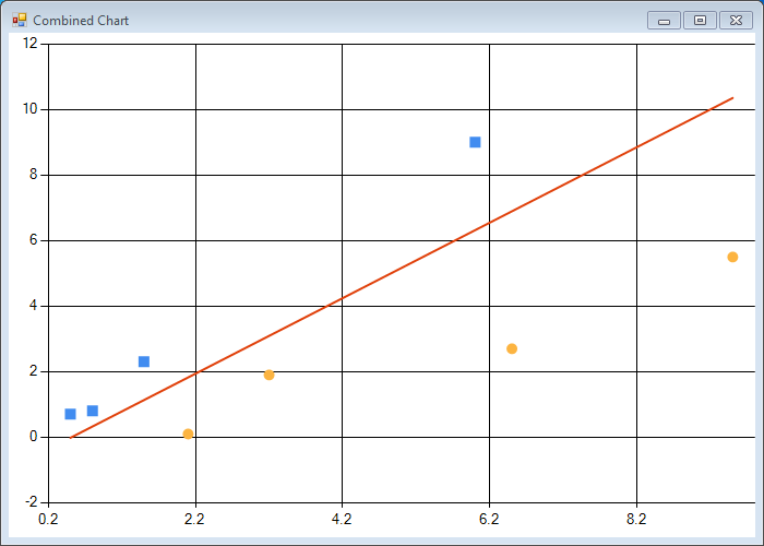
The chart looks reassuring - we get a nice red line, which has the properties we expect: it neatly separates our datasets in two groups based on their label.
Less simple implementation
So far I have followed pretty closely the implementation proposed in Chapter 5. Peter Harrington then proposes an improved implementation, which focuses on improved convergence, by doing two things:
- instead of using a constant alpha, progressively reduces it, which will mechanically reduce the rate of change in the weights vector,
- instead of updating weights by sequentially iterating over the observations, update in random order, which I think is intended to avoid fluctuations in the estimates, if the data is not initially in a random order.
Rather than follow strictly the book’s implementation, I took some liberty, and made some changes, which seemed sensible to me, but could well have some flaws (criticism welcome!).
I modified the approach in 2 minor ways, and a potentially more significant one. First, I modified the mechanism to update alpha; instead of reducing it after each observation, I decided I would work by passes. Each time the algorithm completes a cycle over the entire dataset, alpha is reduced (cooled down) by 10%, with a lower bound it will never pass. Then, instead of using a strict shuffle of the observations after each pass, I decided to simply randomly sample the dataset. The obvious benefit is simplification, the limit being that in a given pass the algorithm will likely be visiting multiple times the same observation, and ignoring some observations. My assumption is that on a large and non pathological dataset, this should have little impact.
The more significant change is that instead of a fixed number of iterations, which is somewhat arbitrary, I decided to try a fixed-point approach: if, after an entire pass, the weights have changed by less than a user-defined epsilon, the search stops. The advantage here is that the termination criterion is less arbitrary - the potential issue being that there could be some convergence issues.
Without further ado, here is the code I ended up with:
// 2-Norm of Vector (length)
let norm (vector: float list) =
    vector |> List.sumBy (fun e -> e * e) |> sqrt

// rate of change in the weights vector,
// computed as the % change in norm
let changeRate before after =
    let numerator =
        List.zip before after
        |> List.map (fun (b, a) -> b - a)
        |> norm
    let denominator = norm before
    numerator / denominator

// recursively updates weights until the results
// converges and weights remains within epsilon
// distance of their value within one pass.
// alpha is progressively "tightened", and
// observations are selected in random order,
// to help / force convergence.
let train (dataset: (float * float list) seq) epsilon =

    let dataset = dataset |> Seq.toArray
    let len = dataset |> Array.length
    let cooling = 0.9
    let rng = new Random()
    let indices = Seq.initInfinite(fun _ -> rng.Next(len))

    let rec descent curWeights alpha =
        let updatedWeights =
            indices
            |> Seq.take len
            |> Seq.fold (fun w i ->
                let (label, observ) = dataset.[i]
                update alpha w observ label) curWeights
        if changeRate curWeights updatedWeights <= epsilon
        then updatedWeights
        else
            let coolerAlpha = max epsilon cooling * alpha
            descent updatedWeights coolerAlpha

    let vars = dataset |> Seq.nth 1 |> snd |> List.length
    let weights = [ for i in 0 .. vars -> 0.0 ] // 1 more weight for constant

    descent weights 1.0
We define the norm of a vector (its length), and the changeRate between two vectors as the ration of the distance of their difference, divided by the norm of the original vector. The train function now takes in a dataset, and a variable epsilon, the percentage change in weights which once reached will stop the algorithm. Inside the train function, we create an infinite sequence of random integers, which will return random indices of observations in the dataset. The rest of the function is fairly similar in spirit to the previous version, except that for each pass we now pick random observations instead of sequential ones, and keep iterating and cooling down alpha until the changes in weights become less than epsilon.
Comparison
So how does the algorithm perform on larger datasets? Let’s check out in our script.
let rng = new System.Random()
let w0, w1, w2, w3, w4 = 1.0, 2.0, 3.0, 4.0, -10.0
let weights = [ w0; w1; w2; w3; w4 ] // "true" vector
let sampleSize = 10000

let fakeData =
    [ for i in 1 .. sampleSize -> [ for coord in 1 .. 4 -> rng.NextDouble() * 10.0 ] ]

let inClass x = if x <= 0.5 then 0.0 else 1.0

let cleanLabels =
    fakeData
    |> Seq.map (fun coords -> predict weights coords)
    |> Seq.map inClass

let noisyLabels =
    fakeData
    |> Seq.map (fun coords ->
        if rng.NextDouble() < 0.9
        then predict weights coords
        else rng.NextDouble())
    |> Seq.map inClass

let quality classifier dataset =
    dataset
    |> Seq.map (fun (lab, coords) ->
        if lab = (predict classifier coords |> inClass) then 1.0 else 0.0)
    |> Seq.average
We define an arbitrary set of weights, and create a sample of 10,000 datapoints in [0; 10] x [0; 10]. We then create two datasets, a clean set and a noisy set. The clear set assigns to each point its correct class, by using the predict function. The noisy set assigns each point a random label instead of the correct one with a 10% probability, so about 5% points should be mis-classified. Note that while 5% is not too high of a proportion, these could be complete outliers, because the misclassification is completely unrelated with the actual position of the point, and whether or not it is close to the separating plane.
Finally, we define a quality function, which takes a classifier and a dataset, counts every point which is properly classified, and averages out the result, which produces the proportion of properly classified points.
We can now compare the two training methods, on both datasets:
printfn "Clean dataset"
let cleanSet = Seq.zip cleanLabels fakeData
printfn "Running simple training"
let clean1 = simpleTrain cleanSet 100 0.1
printfn "Correctly classified: %f" (quality clean1 cleanSet)
printfn "Running convergence-based training"
let clean2 = train cleanSet 0.000001
printfn "Correctly classified: %f" (quality clean2 cleanSet)

printfn "Noisy dataset"
let noisySet = Seq.zip noisyLabels fakeData
printfn "Running simple training"
let noisy1 = simpleTrain noisySet 100 0.1
printfn "Correctly classified: %f" (quality noisy1 noisySet)
printfn "Running convergence-based training"
let noisy2 = train noisySet 0.000001
printfn "Correctly classified: %f" (quality noisy2 noisySet)
Given the random nature of the dataset, results will vary. This is what I got on my machine:
>
Running simple training
Correctly classified: 0.998200
Real: 00:00:03.565, CPU: 00:00:03.546, GC gen0: 386, gen1: 1, gen2: 0

val cleanSet : seq<float * float list>
val clean1 : float list =
  [6.412178103; 11.98456177; 18.67679026; 25.08910831; -62.06700591]

>
Running convergence-based training
Correctly classified: 1.000000
Real: 00:00:02.493, CPU: 00:00:02.484, GC gen0: 263, gen1: 1, gen2: 0

val clean2 : float list =
  [22.00875325; 43.28588972; 64.84288882; 86.24888736; -215.9182689]
On the clean set, both approaches perform comparably well, with a speed advantage for the new version. This is the intended benefit of the convergence-based approach: why keep iterating, if the search doesn’t produce anything different? Interestingly, the weight vectors are co-linear, but on different scales.
How about the noisy set?
>
Running simple training
Correctly classified: 0.818300
Real: 00:00:03.604, CPU: 00:00:03.593, GC gen0: 375, gen1: 2, gen2: 1

val noisySet : seq<float * float list>
val noisy1 : float list =
  [1.738595354; 0.9666423757; 0.8632194661; 1.090752279; -2.66961749]

>
Running convergence-based training
Correctly classified: 0.945600
Real: 00:00:04.742, CPU: 00:00:04.750, GC gen0: 504, gen1: 0, gen2: 0

val noisy2 : float list =
  [0.4489143265; 0.20478143; 0.3220200493; 0.4090429293; -1.102862438]
This time, there is a slight time advantage to the simple training method, but the new method performs much better in terms of classification, getting as good a result as could be expected, given that an expected 5% of the points should be mis-classified in the dataset. The other observation is that the weight vectors identified by the algorithm are much further from the true underlying weights - but the new method produces something much closer to the expected result (rescaling notwithstanding).
Conclusion
My impression on Logistic Regression is that the stochastic descent implementation was, once again, extremely straightforward in F# - under 100 lines of code without comments. The algorithm itself runs pretty fast, and is fairly simple to follow, but I was surprised by the quick degradation of results once noise is added to the dataset. I assume this has to do with the way I modeled noise, as completely independent of the actual position of the point itself; a quick-and-dirty experimentation with points mislabeled based on proximity to the separating plane yielded much better results.
In any case, I hope you found this interesting or even useful - and I’d love to hear your comments or criticisms!
Additional resources
- Code on GitHub
- the code presented in the post is available in the LogisticRegression.fs module and the Chapter5.fsx script file.
Coding Logistic Regression with Newton-Raphson: MSDN Magazine article presenting a C# implementation with deterministic gradient.